Getting Started
This tutorial builds a small two-dimensional B-scan model, runs gprMax through
GprMaxModel, and inspects the output.
Imports
 1
 2
 3
 4
 5
 6
 7
 8
 9
10
11
12
13
14
15
16
17
18
19 | from pathlib import Path
from gprmaxui import GprMaxModel
from gprmaxui.commands import (
DomainBox,
DomainResolution,
DomainSize,
DomainSphere,
HertzianDipole,
Material,
Rx,
RxSteps,
SrcSteps,
TimeWindow,
Tx,
TxRxPair,
Waveform,
)
from gprmaxui.utils import make_images_grid
|
Create the Model
GprMaxModel stores the domain definition, output folder, simulation time, and
commands that will be written to a gprMax input file.
| model = GprMaxModel(
title="B-scan from a single target buried in a dielectric half-space",
output_folder=Path("output"),
domain_size=DomainSize(x=0.2, y=0.2, z=0.002),
domain_resolution=DomainResolution(dx=0.002, dy=0.002, dz=0.002),
time_window=TimeWindow(twt=3e-9),
)
|
Register Materials and Geometry
Materials are registered first, then referenced by geometry objects.
1
2
3
4
5
6
7
8
9
10
11
12
13
14
15
16
17
18
19
20
21
22
23 | model.register_materials(
Material(id="half_space", permittivity=6, conductivity=0, permeability=1)
)
box = DomainBox(
x_min=0.0,
y_min=0.0,
z_min=0.0,
x_max=0.2,
y_max=0.145,
z_max=0.002,
material="half_space",
)
model.add_geometry(box)
target = DomainSphere(
cx=box.center().x,
cy=box.center().y,
cz=box.center().z,
radius=0.005,
material="pec",
)
model.add_geometry(target)
|
Add a Source and Receiver
Tx binds a waveform to a source command. TxRxPair combines that transmitter,
the receiver, and the step increments used when gprMax runs multiple traces.
 1
 2
 3
 4
 5
 6
 7
 8
 9
10
11
12
13
14
15 | tx_rx_sep = 2e-2
tx = Tx(
waveform=Waveform(wave_family="ricker", amplitude=1.0, frequency=1.5e9),
source=HertzianDipole(polarization="z", x=0.03, y=0.15, z=0.0),
)
rx = Rx(x=tx.source.x + tx_rx_sep, y=0.15, z=0.0)
model.set_source(
TxRxPair(
tx=tx,
rx=rx,
src_steps=SrcSteps(dx=0.002, dy=0.0, dz=0.0),
rx_steps=RxSteps(dx=0.002, dy=0.0, dz=0.0),
)
)
|
Run the Simulation
Use n="auto" when the trace count should be inferred from the receiver
position, domain width, and receiver x-step.
| model.run(n="auto", geometry=True, snapshots=True)
|
Note
Snapshot output can become large. For longer runs, use
snapshot_stride to save only every nth simulation iteration.
Read Output Data
model.data() returns a dictionary keyed by receiver component. Each value is a
tuple containing the B-scan array and the model time step.
| data = model.data(rx=1)
ez_data, dt = data["Ez"]
print(ez_data.shape, dt)
|
Save and Reload a Model Configuration
Version 1.0.3 supports Pydantic-backed JSON export and import for reusable
model definitions. This stores the model title, output path, domain, time
window, source, materials, and geometry commands.
| model.to_json("single_target_model.json")
restored_model = GprMaxModel.from_json("single_target_model.json")
|
To keep the JSON in memory:
| model_json = model.to_json()
restored_model = GprMaxModel.from_json(model_json)
|
Visualize Results
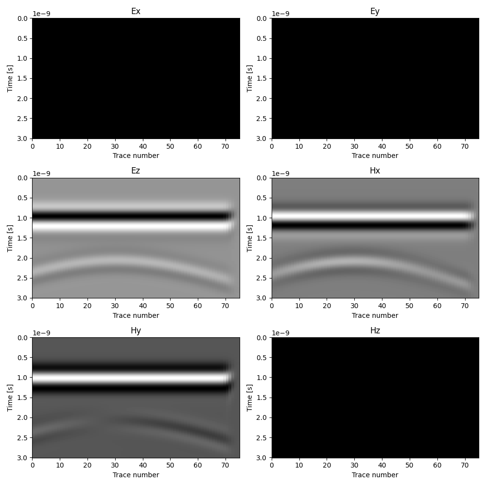
| model.plot_data()
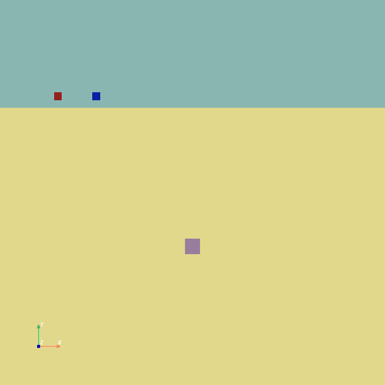
model.plot_geometry()
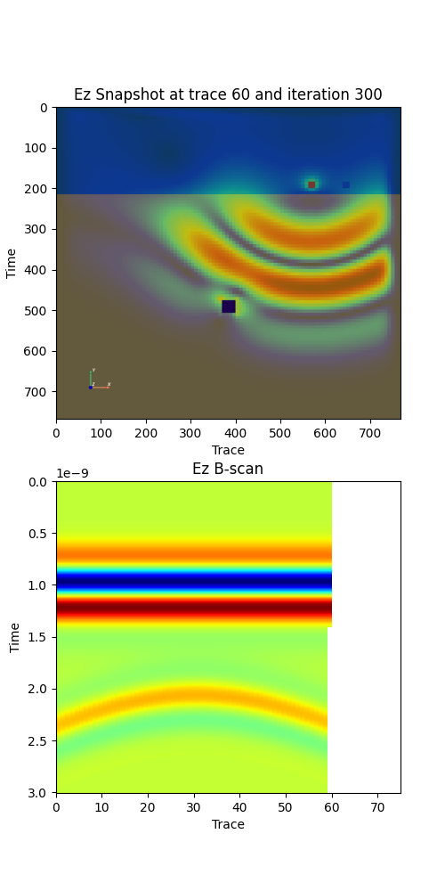
model.plot_snapshot(trace_idx=60, iteration_idx=300)
|
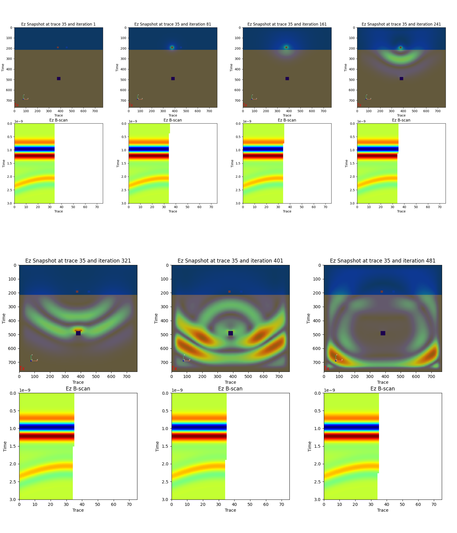
To compare several simulation times, collect returned images and assemble them
into a grid.
1
2
3
4
5
6
7
8
9
10
11
12 | captures = []
for iteration_idx in range(1, 500, 80):
captures.append(
model.plot_snapshot(
trace_idx=35,
iteration_idx=iteration_idx,
return_image=True,
)
)
output_image = make_images_grid(captures, num_cols=4)
output_image.show()
|